User Interface Overview
AGAVE is a windowed desktop application.
The application is divided into several panels. All of the panels except for the 3D view can be undocked by dragging their title bar with the mouse. Undocked panels can float independently or the interface can be reconfigured by re-docking them in a different position. Note: currently, restarting AGAVE will reset the interface to the default configuration.
All panels can be resized by dragging from their edges. Your cursor should change to indicate when you are hovering over an edge that can be resized.
Tip: On some screens, the panels may be too narrow to have enough range to move the horizontal sliders. In that case, it can help to un-dock the panel and stretch it wider.
If you close any panels, you can always reopen them from the View menu.
Loading volume data
AGAVE can load multi-scene, multi-time, and multi-channel files. It can present up to 4 channels concurrently and offers a time slider when time channels are detected.
Metadata embedded in the file is important for AGAVE to display the volume properly. AGAVE can decode OME metadata (OME-TIFF files), ImageJ metadata (TIFF files exported from ImageJ/FIJI), Zeiss CZI metadata, and OME-Zarr metadata.
We recommend preparing or converting your volumetric files to OME-TIFF or OME-Zarr (see Preparing an AGAVE Compatible ome-tiff file with Fiji to ensure the expected data structure, channel order, etc.)
AGAVE currently supports the following file formats: * .zarr (OME-Zarr only - https://ngff.openmicroscopy.org/latest/) * .ome.tiff (see https://docs.openmicroscopy.org/ome-model/latest/) * .tiff * .czi (Produced by Zeiss microscopes. See https://www.zeiss.com/microscopy/en/products/software/zeiss-zen/czi-image-file-format.html) * .map/.mrc (Typically used in electron cryo-microscopy. See https://www.ccpem.ac.uk/mrc_format/mrc_format.php) AGAVE can read 8-bit, 16-bit unsigned, or 32-bit float pixel intensities.
OME-Zarr data is not stored as single files - instead it is a directory. AGAVE can load OME-Zarr data either from a local directory or from a public cloud URL using https, s3, or gc protocols.
Open file, directory or URL
File–>Open file or [Open file] toolbar button File–>Open directory or [Open directory] toolbar button File–>Open from URL or [Open from URL] toolbar button
[Open file] will pop open a file browser dialog in which you can navigate to the volume file of choice. Check the “Image Sequence” checkbox if your directory contains a time sequence of individual TIFF files. [Open directory] will pop open a directory browser dialog in which you can navigate to the OME-Zarr store of choice. [Open from URL] will pop open an input dialog in which you can enter the URL to the OME-Zarr store of choice. Currently only publicly accessible URLs are supported.
Once the data source location (file, directory or URL) is selected, if the data is multi-scene, a dialog will pop up to let you select the scene you wish to view. To view a different scene, just re-open the same data location.
If the data you select cannot be opened or loaded for any reason, an error dialog will pop open to notify you. There are several possible reasons why this operation may fail and if AGAVE can determine the reason, it will be displayed in the AGAVE log.
One the data source has been selected, the Load Settings dialog will then appear to let you finalize choices for the data to be loaded.
Open JSON
File–>Open JSON or [Open JSON] toolbar button
[Open JSON] can be used when you have previously saved an AGAVE session. This will load the volume file associated with that session, along with all of the AGAVE settings as they were when you saved (if you encounter problems, see Save JSON below for details about proper file and filepath structure).
Recent
File–>Recent…
This menu will present a list of the most recently opened volume files for quick selection if AGAVE was previously used on your computer. This choice will then open the Load Settings dialog.
Load Settings
In order to support loading from very large datasets, AGAVE can load subsets of data based on precomputed multiresolution levels stored in the data, time series, channels, and in some cases sub-regions within the spatial volume data.
OME-Zarr supports all of the above selections when present in the data. Other formats are more restrictive and may only support a few of the options. The Load Settings dialog presents you with a memory estimate of how much data will be loaded with current settings. Coupled with knowledge of your own system’s configuration, this allows you to make informed choices about how much data to load. The memory estimate is an expected estimate of how much GPU memory AGAVE will use for rendering. Main memory usage may be higher, but is not indicated as usually GPU memory is the limiting factor.
Resolution Level
The OME-Zarr format supports precomputed multiresolution data and will let you select the resolution level. The highest resolution is the default, so beware if you have a large dataset, you risk running out of memory.
Time
If you are loading time-series data, you may select the initial time to load. You will be able to change the current time point after the data is loaded. (See Time Panel)
Channels
You may choose to exclude certain channels from being loaded. All channels will be selected by default. If you leave channels out, be aware you will have to reload the file to get them back.
Subregion
For OME-Zarr data, you may select a sub-region in X, Y, and Z. This is useful for loading a subset of a large dataset. A typical usage might be to first load a very low resolution level and then select a sub-region of interest to then load at a higher resolution.
Keep Current AGAVE Settings
If you have already loaded a volume file and have made changes to the appearance, channel intensities, lighting, etc., you can choose to keep those settings when loading a new volume file. This is useful if you are loading several images consecutively that have similar channels and dimensions, and want to apply a consistent appearance to each.
Adjusting the camera view
The 3D viewport in AGAVE supports direct manipulation by zoom, pan, and rotate. It also provides a toolbar with some convenient buttons for common view settings.
Rotate
To rotate the volume, left-click and drag the mouse.
Zoom
To zoom in or out, right-click and drag up or down. On Mac trackpad, Command-click and drag up or down, or drag up or down with two fingers as if scrolling.
Pan
To slide the camera parallel to the screen, middle-click and drag in the view. On Mac, Option-click and drag in the view.
 Reset
Reset
The [Reset] button in the toolbar will return your camera to the default view position as if the volume were freshly loaded.
 Frame View
The [Frame View] button in the toolbar will frame the volume data in the window. This is useful if you have zoomed or panned away from the volume data and want to quickly return to a view that shows the entire volume, but keep the rotation angle.

 Perspective/Orthographic
The [Persp/Ortho] toolbar button will toggle between a perspective projection and an orthographic one. In a perspective projection, parallel lines will meet in the distance and 3D objects will be foreshortened. This is considered a “realistic” view. In orthographic projection, parallel lines receding into the distance will remain parallel no matter which direction they go. There is no foreshortening or tapering of the volume.
 Quick Views


The [Quick Views] toolbar button will pop open a menu of quick views that will automatically rotate the volume to a particular angle. The views are Front, Back, Top, Bottom, Left, and Right to align your viewport perfectly looking along the X, Y or Z axes from either direction.
 Show axes
The [Show axes] toolbar button will toggle the display of the X,Y,Z coordinate axes in the lower left corner of the viewport.
Appearance Panel
The appearance panel has the majority of the controls you will use to adjust the image. In particular, you will adjust volume channel intensities and colors, control how transparent or opaque the volume appears, and control lights and shadows.
Global Rendering Settings
Renderer
Select [Path Traced] for the standard high quality rendering system. Select [Ray March Blending] for a faster performing but simplified renderer. The Ray Marching renderer will not do advanced lighting and shadowing, but can still provide a useful view of your volume data. It does not behave in a progressive fashion, instead giving you the finished image immediately with no waiting.
Scattering Density
Scattering density controls how dense (opaque) or sparse (translucent) the volume appears. Higher density can be helpful for objects with well defined edges and less noisy data. It also tends to bring out the lighting in a more pronounced way. Lower density can be useful for multichannel viewing in which the data has a lot of overlap.
Shading Type
There are two shading methods: [BRDF] and [Phase]. The [Mixed] setting combines the two and is the default. The BRDF (Bidirectional Reflectance Distribution Function) is more sensitive to lighting angle and can produce a shiny reflective appearance, whereas the Phase function does not produce glossy highlights.
Shading Type Mixture
In Mixed shading mode, this slider controls the relative contribution of Phase and BRDF.
Primary Ray Step Size
The primary ray step size controls the distance rays can travel into the volume before hitting something. Larger values will render faster but also result in some rays bypassing important parts of the volume. This can be used for quicker preview rendering. Smaller values will be more precise and ensure that you are capturing every detail in the volume data.
Secondary Ray Step Size
The secondary ray step size controls the distance rays will travel after they have scattered within the volume and are bouncing out toward the light sources. Higher values will brighten the image and reduce shadows because more rays will penetrate through the volume and make it out to the lights. Smaller values will ensure that some rays are stopped by volume data, which will increase the accuracy of cast shadows.
Interpolate
Check this box to enable or disable interpolation between volume pixels. Turning it off will work well for segmentation data or data that has definite discontinuous boundaries. Turning it on (the default) will smooth out the data and make it look more continuous, and can enhance the appearance of raw microscopy image data.
Background Color
Clicking on the color square next to Background Color allows you to change the image background color from black (default) to any other color.
Bounding Box
Click the checkbox to show or hide a bounding box line around the volume data. Clicking on the color square allows you to select a color for the bounding box lines.
Scale Bar
Click the checkbox to show or hide a scale bar at the bottom right corner of the display. In a perspective camera, due to foreshortening, the scale bar will represent the distance between tickmarks shown on the bounding box of the volume. You will have to have the bounding box turned on in order to see it. The scale bar will use physical units if available in the loaded volume data.
Timestamps
For time-series data, you can display the current timepoint as an overlay in the top-right corner of the viewport. Check the “Timestamps” checkbox to turn the overlay on or off.
The “Timestamp Format” dropdown selects how the time is displayed:
HH:MM:SS: the current time is converted to seconds and shown as a clock-style value. Fractional seconds are added automatically when the spacing between timepoints requires them for the value to change visibly.
Time Units: the current time is shown using the physical time units read from the file metadata (for example seconds, minutes, or whatever the data records). The numeric precision adapts to the magnitude of the value so the display stays readable.
If the loaded data has only a single timepoint, the timestamp overlay has nothing to display.
Volume Scale
These X, Y, and Z values describe the physical dimensions of the volume data relative to the number of pixels. Often microscopes do not have the same physical dimensions in Z that they do in X and Y. Usually these values are read from the volume file’s metadata. If they could not be found in the metadata, they will often appear here as X=1, Y=1, Z=1. They can be modified here. Each axis can also be inverted by checking the corresponding “Flip” checkbox.
Region Of Interest (ROI)
Three sliders presented here let you clip the volume along each of its three axes. These sliders have two handles each, which let you clip each dimension from either side. For example, to see only the bottom Z half of your volume (or display the cross section middle slice), move the rightmost Z handle about halfway to the left.
Clip Plane
The clip plane is a plane that can be moved through the volume to cut away sections. The plane can be moved in X, Y, and Z, and rotated to any angle. Check the checkbox to enable or disable the clipping. Check “Hide” to make the clip plane grid indicator disappear. Click “Reset” to return the plane to its initial position. Click “Rotate” or “Translate” to enable viewport controls to let you move the clip plane interactively. Click the Rotate and Translate buttons a second time to disable the viewport controls. See Rotate below for more details.
Lighting
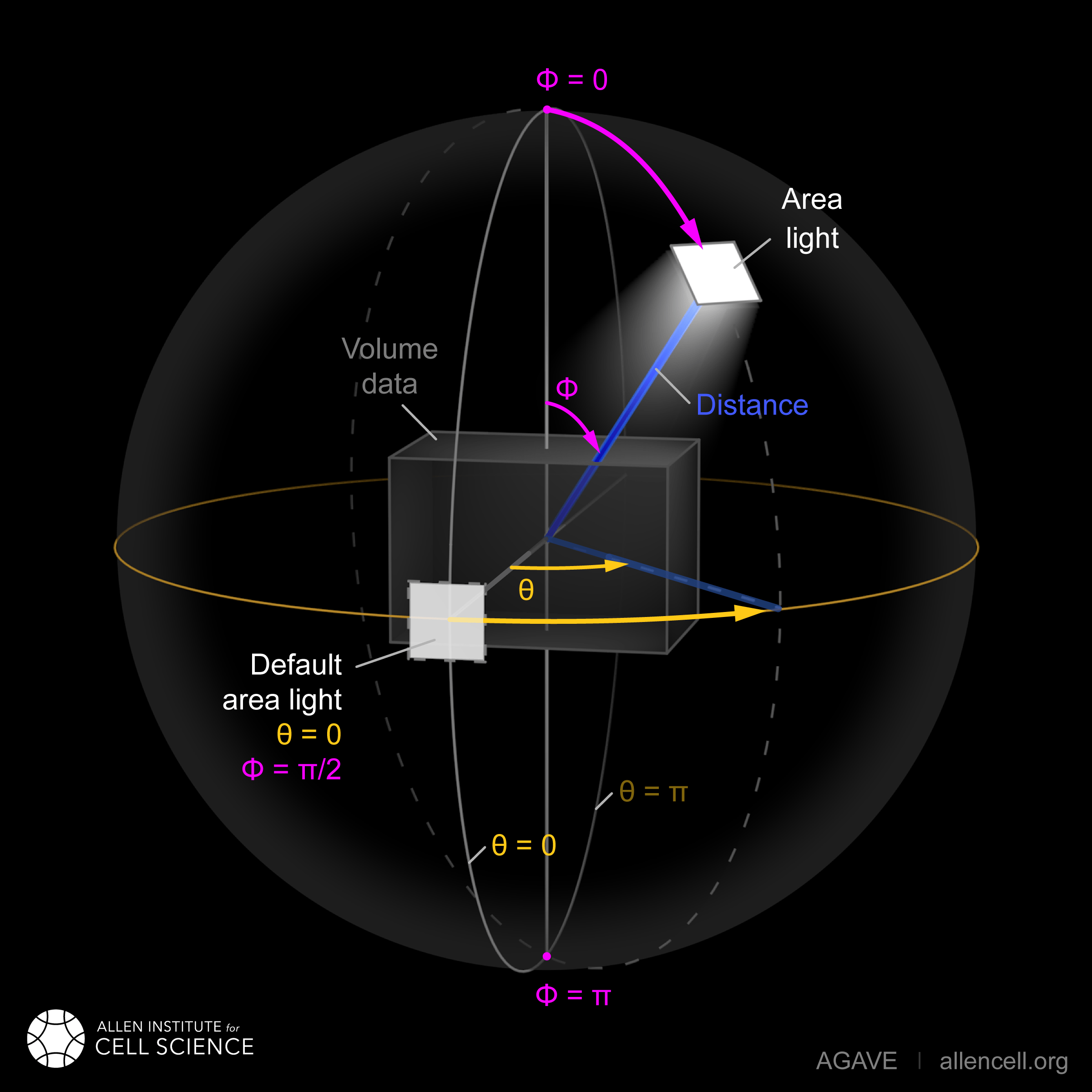
There are two types of light illuminating your volume. One is an “Area Light”, represented by an imaginary square-shaped light source that can be moved anywhere around the volume. The second is a “Sky Sphere”, which can illuminate the volume from all directions.
Each light has a “Rotate” button to enable an interactive manipulator in the viewport (see Rotate below) and a “Reset” button to return that light to its default orientation and settings.
Lock Lights to Camera
This checkbox, which is enabled by default, controls how the lights behave when you rotate the camera in the viewport.
When checked, the lights are locked to the camera, so they keep the same orientation relative to your point of view as you rotate the volume. Think of it as if you were holding a flashlight still while tumbling the volume data in front of you. This keeps the volume evenly lit from your current viewing angle no matter how you turn it.
When unchecked, the lights stay fixed in world space. Rotating the camera then moves your viewpoint around stationary lights, so the same parts of the volume will be illuminated no matter how you rotate the view.
Tip: it can be useful to turn one light off while tuning the settings for the other.
Area Light Theta, Phi, and Distance
These three coordinates let you position the light anywhere on a sphere around the volume. Theta and Phi are in radians (where 3.14159 radians is half a circle).
Rotate
If you click “Rotate”, an interactive rotation widget will appear in the viewport. You can click and drag on the widget to rotate the light direction around the volume. If you click on the colored lines of the axes, rotation will be constrained to that axis. Click “Rotate” again to hide the rotate manipulator.
Area Light Size
The size of the light controls the spread of its illumination over the volume. A smaller light closer to the volume will appear very dramatic with exaggerated shadows, due to its rays spreading over a wide angle. A larger light will give a more even illumination.
Area Light Intensity
You may select a RGB color for the area light, and modify it with a scalar intensity value to brighten or darken it. Note that you can turn the light off by setting its color to black or its intensity to 0.
SkyLight Top, Middle, and Bottom
The Sky Light is described by a sphere completely surrounding the volume. You can set a color and intensity for the “north pole” (Top) of the sphere, the “equator” (Middle) and the “south pole” (Bottom). These values will be interpolated to compute the light at any point in between. The Sky Light can be turned off by setting its intensities to 0 or its colors to black.
Volume Channel Settings
Each volume channel contains adjustable settings. Expand the channel menus to access the following parameters.
Transfer Function Editor
The transfer function editor lets you transform the intensity values in your volume data to clarify and fine-tune your visual analysis. You can select particular intensity ranges to view, to pick out particular details in the volume.
The editor displays a graph at the top. The background of the graph contains a histogram, showing where the volume intensity is distributed (Y axis) along the intensity range (X axis). The white line shows how volume intensities X are remapped to new intensities Y.
The graph itself can be zoomed and panned along the X axis. To zoom, use the mouse wheel (or two finger drag up/down on touchpad). To pan, click and drag the graph. To reset the graph to fit the data, double-click anywhere in the graph area. As you zoom and pan, the histogram’s vertical (Y) axis automatically rescales to fit the data currently in view, so tall peaks elsewhere in the intensity range will not flatten the detail you are looking at.
A “Log” toggle button switches the histogram’s Y axis between linear and logarithmic scaling. Logarithmic scaling makes it easier to see sparse intensities that would otherwise be dwarfed by a few very tall bars. The “Log” button has no effect on the transfer function curve itself, which is always linear between control points.
The editor has 4 mutually exclusive modes. You can switch between any of the modes and each mode’s settings will be remembered.
The “Copy” and “Paste” buttons let you copy the current channel’s transfer function settings and apply them to another transfer function mode within the same channel. (Copy is not available in Custom mode, as Custom mode can involve multiple control points that can’t be translated to the other modes.)
The control modes are described as follows:
Min / Max
Min/Max lets you remap the data range to a narrower range and clip data above and below the selected range. AGAVE provides two controls: a minimum intensity that will be remapped to 0, and a max intensity that will be remapped to 1 (full brightness). You can also click and drag the point handles in the graph directly to adjust the min and max.
Window / Level
Window/Level lets you remap the data range to a narrower range and clip data above and below the selected range. AGAVE provides two controls: one to define how wide the range is (the window), and another to control where the window lies in the raw intensity range (the level). You can also click and drag the point handles in the graph directly to adjust the window and level.
Isovalue
Isovalue lets you select a range of intensity values and clips all other values to 0. You may select a middle intensity value and a range of values above and below it. A thinner range will let you isolate one particular intensity.
Histogram Percentile
Percentile mode is similar to Window/Level as it results in the same linear remapping, but the choice of start and end is based on a percentage of the total pixels in the image. The default is to clip the bottom 50% of pixels to zero, and clip the upper 2% of pixels to maximum. You can also click and drag the point handles in the graph directly to adjust the percentiles.
Custom
In Custom mode, you are free to edit the graph yourself. You will create your own piecewise linear transfer function. You start by default with a 1-1 intensity remapping, with one point in the bottom left corner and another in the upper right. Click in the graph anywhere to create a new vertex. It will be represented by a white circle. Click the middle of a circle and drag to move it.
Behavior on time change
When you change the current time in the Time Panel, the transfer function is updated to keep your settings meaningful against the new timepoint’s histogram. The behavior depends on the active mode:
Min/Max, Window/Level, Isovalue, and Custom: the control points are preserved at the same absolute intensity values. If the new timepoint has a different data range, the underlying parameters (window, level, isovalue, custom control point positions) are recomputed so that the same raw intensities continue to be selected. This keeps the rendered image visually stable across timepoints.
Histogram Percentile: the percentile values are preserved instead of the absolute intensities. The transfer function is recomputed from those percentiles against the new timepoint’s histogram, so it adapts to changes in the intensity distribution from frame to frame.
The histogram bars in the graph are always redrawn to reflect the new timepoint’s data.
Color settings
ColorMap
The colormap is a gradient that maps intensity values to colors. You can select from a variety of built-in colormaps. The color map will be applied between the min and max values of the transfer function. If you are using a “Custom” transfer function then there may be no inherent min and max. In this case, the color map will be applied to the whole data range. To disable the color map, select the first entry (labeled as “none”). If your data is discrete labels such as a segmentation, you may use the final entry in the list, “Labels”, which will assign a unique color to each unique intensity value. Note that the colormap colors will be multiplied with the [Color] setting. Set Color to white to see the colormap directly.
Color
This should be thought of as the main color for this channel. Set this to white in order to use the color map without any extra color tinting.
Specular Color
This is the color for reflective highlights. It is additive on top of the diffuse color. Leave it at black to have no shiny highlights at all. This color should be tuned in conjunction with the Glossiness slider.
Emissive Color
This color is not truly light-emitting, but can not be darkened by the effects of shadowing from other lights. It should be used sparingly, if at all.
Glossiness
The glossiness value controls how sharp the reflected Specular highlights are. It defaults to a low value which makes them seem more diffuse. Higher values will appear shinier or glossier.
Output: Saving Results
Quick Render
File–>Quick render or the [Quick render] toolbar button
Save the current viewport window as a PNG, or JPG file.
Render
File–>Render or the [Render] toolbar button
Opens the Render Dialog
Save JSON
File–>Save to JSON or [Save to JSON] toolbar button
Save to JSON will save the current AGAVE session into a small file that records every setting so you can pick up work where you left off. The JSON file is a text file, which you can (carefully) hand-edit if you need to. The file name of the currently loaded volume file is embedded in the JSON, so if you copy the file around you should bring the volume data file with it. It is best to keep them in the same directory if possible.
Save To Python Script
File–>Save to Python script or [Save to Python script] toolbar button
Save to Python script will save the current AGAVE session into a small Python file. See [Python Interface] for how to use the Python programming language to automate AGAVE to create animation sequences or batch rendering of many images.
Render Dialog
The Render dialog lets you control various quality settings for output of your final image. It also allows you to orchestrate time series batches. Hint: Quick Render is the best way to just get a snapshot of your 3D viewport. Render is for when you want to more carefully control output resolution and quality. Progress bars for single image and time series rendering are displayed at the bottom of the dialog.
Image preview
The preview window will update during rendering with the current image as it is being computed. Left-button drag in the view to pan the image. There are three tool buttons to let you zoom in (“+”), zoom out (“-“), and frame the image to the preview window (“[]”). When you stop rendering and start changing any output resolution parameters, the image will reset to a checkerboard.
Output Resolution
Choose the number of pixels for the final rendered image. By default, the X and Y values are linked to maintain the same aspect ratio. Changing one will cause the other to change automatically. Toggle the link icon to allow them to change independently.
Several Resolution Presets are offered as a convenience to quickly select commonly used output resolutions.
Image Quality
You can choose to control the final image quality by specifying either number of Samples per pixel, or how much Time to spend rendering. Higher values will result in higher quality. AGAVE computes its final image by gathering samples iteratively. For a quick preview render, you can set the number of samples to a low value such as 32. For a final image, you can set the number of samples to a high value such as 1024. The contribution of each sample will be less than the previous sample. Therefore you may get subtle but important improvements in quality well beyond 1024 samples. The rate at which each sample is gathered is completely dependent on the performance characteristics of your computer. If you prefer to simply have a time budget, you may also choose to select Time and specify how long to render. The renderer will gather as many samples as possible within the specified time.
Output File
Here you can select the output directory and a name for the output file. AGAVE currently only renders to PNG file format. If you are rendering a time series, AGAVE will append “_0000”, “_0001”, etc. to the file name for each frame. For time series, if the file you are rendering already exists, AGAVE will prompt you to overwrite it. If you are rendering only a single frame, AGAVE will append a number to the file name if the file already exists.
Camera Panel
The camera panel controls will let you affect the image’s exposure amount, and control the focus blurring.
Exposure
The exposure value will brighten or darken the overall image.
Exposure Time
This setting should normally be kept at 1, but if you have a sufficiently powerful GPU, increasing it will render more paths before refreshing the view, and make the image resolve faster. Only change this if your image already resolves very quickly.
Noise Reduction
Noise reduction applies a filter to the image to reduce the graininess of early render passes. After the image has resolved beyond a certain level, the denoiser will shut off and have no effect. The image will continue to accumulate samples and resolve via brute force computation.
Aperture Size
Aperture size affects the depth of focus, or how much of the image is in focus. A small aperture size will keep the entire image in focus at all times. A large aperture size will let you only focus on a thin plane a specific distance from the camera.
Field of View
The field of view is an angle in degrees describing how narrow or wide an angle your camera can cover. A smaller field of view will span a very small section of your volume and will give the impression of zooming in while at the same time reducing the perspective foreshortening. A large field of view will have increased perspective distortion and give the impression of zooming out as the camera angle can show more and more of the scene being displayed.
Focal Distance
Focal distance describes the distance from the camera lens that is the center of focus. For aperture size 0, this has no effect, since the entire image will remain in focus (effectively an infinite focus depth range).
Time Panel
For time series data, move the time slider or change the numeric input to load a new time sample. Beware that this is loading a whole new volume and can take some time. Nothing will be loaded while dragging the slider; AGAVE will load the new time sample when the slider is released or the numeric input is incremented. If your dataset only has a single time, then the Time Panel will be hidden.
When a new timepoint is loaded, each channel’s transfer function is automatically updated against the new histogram. For most modes the absolute intensity thresholds are preserved; in Histogram Percentile mode the percentile values are preserved and the thresholds are recomputed. See Transfer Function Editor (Behavior on time change) for full details.
Python Interface
AGAVE can be automated and controlled via Python when it is launched in server mode from the command line. First, install the AGAVE Python client:
pip install agave_pyclient
The Python client will then find a running AGAVE server session and send
commands to it. The AgaveRenderer will automatically launch a local AGAVE server
for you if it cannot find one already running (see the
agave_pyclient documentation
for the auto_launch and agave_path options).
A Python script exported from the AGAVE GUI using “Save to Python script” will re-create the session and produce an image when run.
python my_script.py
Scripts exported from AGAVE in this way will automatically launch an AGAVE server if one is not already running, so you can run them without any special setup.
To run AGAVE as a server explicitly, run:
agave --server
The AGAVE Python client provides commands for every setting in the user interface, and also provides two additional convenience commands for creating an image sequence for a turntable rotation, and for a rocker (side to side) rotation. For Python users, the AGAVE Python client project full documentation can be found here: https://allen-cell-animated.github.io/agave/agave_pyclient
Command Line Interface
AGAVE supports the following command line options:
--server
Runs AGAVE without opening a window. AGAVE will wait for a local websocket connection on port 1235 by default. See Python Interface for more information about how to communicate with AGAVE in server mode.
--port number
Specifies the port to listen on in server mode. Defaults to 1235. A port given here overrides any port specified in a
--configfile.
--config filepath
Provides a JSON configuration file for server mode that contains a custom port number. Filepath is defaulted to setup.cfg. The JSON must be of the form
{ port: portnumber }.
--load fileOrUrl
Opens the given file or URL on startup. This works both in windowed mode and in server mode.
--list_devices
Only valid in server mode on Linux. AGAVE will dump a list of possible GPU devices and then exit.
--gpu number
Only valid in server mode on Linux. Selects a device to use from the list provided by list_devices. The device is specified as a zero-based index into the list.
-platform offscreen
Only valid in server mode on Linux. Allows AGAVE to run as a server on a headless cluster node. On other platforms AGAVE must be run in a windowed desktop environment, even in server mode.
Citation
Daniel Toloudis, AGAVE Contributors (2026). AGAVE: Advanced GPU Accelerated Volume Explorer (Version 1.10.0) [Computer software]. Allen Institute, Cell Science. https://github.com/allen-cell-animated/agave
bibtex:
@software{agave,
 author       = {Toloudis, Daniel and AGAVE Contributors},
 title        = {AGAVE: Advanced GPU Accelerated Volume Explorer},
 year         = {2026},
 version      = {1.10.0},
 url          = {https://github.com/allen-cell-animated/agave},
 organization = {Allen Institute, Cell Science},
 note         = {Computer Software}
 }
Troubleshooting
AGAVE Log
The AGAVE log is a plain text stream of informational output from AGAVE. It can be found in the following locations:
Windows: C:\Users\username\AppData\Local\AllenInstitute\agave\logfile.log
Mac OS: ~/Library/Logs/AllenInstitute/agave/logfile.log
Linux: ~/.agave/logfile.log
For troubleshooting, it can be useful to refer to this file or send it with any communication about issues in AGAVE.
Preparing an AGAVE Compatible ome-tiff file with Fiji
Use Fiji to combine volume channels together into a single multichannel file:
File->Import->BioFormats
To convert an existing multichannel file to ome-tiff select a multichannel file, e.g .czi or similar
To convert multiple single channel files into a compatible ome-tiff open all the tiff stacks in FIJI as separate images at the same time. (this assumes each tiff is a z-stack representing one channel, and all the Tiffs have the same X,Y,Z dimensions)
When using Import->BioFormats, make sure “Hyperstack” and “Split Channels” is checked.
Ensure every channel is 16-bit using Image->Type->16-bit
Image->Colors->Merge Channels
select each channel one by one in the dialog that opens.
uncheck [ ] Create composite
Click OK
File->Save As (select ome-tiff)
Note that the channel names will not be saved!
To Open in AGAVE see the Open Volume section above.